Advanced Histogram Plotting

In the previous section, we saw how to contruct histogram plots of magnitude, direction/orientation and both. In this page, we’ll see an easier way to produce these plots, as well as other types of advanced plots that we can construct to further analyse our data.

We’ll use the same dataset as in the previous example, which we’ll load from the NumPy file two_clusters.npy right now. As we mentioned before, these vectors are bundled in the data module, as SampleData.TWO_CLUSTERS and so we can access them without downloading any extra files.

Attention

You probably know this by now, but don’t forget to import VectoRose into your Python shell by writing import vectorose as vr.

import vectorose as vr
import vectorose.data

my_vectors = vr.data.SampleData.TWO_CLUSTERS.load()
my_vectors = vr.util.remove_zero_vectors(my_vectors)

my_vectors

array([[ 0.01330902,  0.06486094, -0.08154041],
       [ 0.19911095,  0.06809676, -0.02230348],
       [ 0.14568445,  0.08995054,  0.06688315],
       ...,
       [-0.0377645 ,  0.35891606,  0.6731566 ],
       [-0.13033349,  0.56234415,  0.27104764],
       [-0.03287074,  0.60723468,  0.63249369]], shape=(200000, 3))

We now have our vectors loaded and we can begin constructing our histograms.

Some Statistics Terminology

VectoRose is designed to analyse collections of vectors having a magnitude that is not necessarily 1. We analyse collections of non-unit vectors or axes, as we explained in the Introduction to Vectors section. When converting to spherical coordinates, we break these vectors down into two different sets of numbers: the magnitudes and the directions or orientations. These two quantities are separate but linked through some external process. By combining these two variables, our non-unit vectors are bivariate. When we consider the nested spheres plot, we are looking at a bivariate histogram, showing both the magnitude of the vectors (which shell the vector falls into) and the direction of the vectors (which patch the shall the vector falls into). This histogram may also be referred to as the joint histogram.

As we saw before, we can construct histograms of the magnitude and the orientation separately. These are known as the marginal histograms. In these cases, we consider only the magnitudes or the directions of the vectors, and we completely ignore the other variable.

But what if we don’t want to completely ignore the other variable? What if we only want to know the directions in which the largest-magnitude vectors are pointing? Or what if we want to know what magnitudes are present in a given direction? The answer is the conditional histogram. In a conditional histogram, we fix the value of one of the variables and study how the other one changes within the selected data. For example, if we want to study the directions of the largest-magnitude vectors, we can simply select all the vectors with a magnitude above certain threshold and then study their directions, ignoring the low-magnitude vectors. Similarly, to study the magnitudes of the vectors in a certain direction, we may select only the vectors in that direction, and then study their magnitudes.

VectoRose allows easy construction of bivariate/joint, marginal and conditional histograms based on vectorial and axial data. In this section, we’ll see how to build each of these histograms, while the next section will introduce quantitative statistics that can be computed for direction and orientation on these distributions.

Some Setup

For all our histograms, we need to have an instance of a subtype of SphereBase. The exact same steps work regardless of which sphere discretisation we use. We can use either TriangleSphere or one of our TregenzaSphere types. In this case, we’ll use a FineTregenzaSphere. To appreciate the magnitude distribution, we’ll consider 32 shells.

my_sphere = vr.tregenza_sphere.FineTregenzaSphere(number_of_shells=32)

This sphere object will be important to all our downstream tasks. Let’s also assign all our vectors to the correct histogram bins using SphereBase.assign_histogram_bins().

labelled_vectors, magnitude_bins = my_sphere.assign_histogram_bins(my_vectors)

labelled_vectors

	phi	theta	magnitude	shell	ring	bin
0	140.922763	11.595749	0.105038	2	41	3
1	96.050088	71.119103	0.211612	4	28	34
2	68.662637	58.307407	0.183816	3	20	26
3	108.637973	58.402654	0.283404	5	32	26
4	101.600750	38.565368	0.301634	6	30	18
...	...	...	...	...	...	...
199995	70.754479	309.190779	0.922267	18	21	141
199996	35.055502	350.961121	0.900928	18	11	101
199997	28.196955	353.993542	0.763798	15	9	85
199998	64.847612	346.951053	0.637718	12	19	151
199999	43.874659	356.901498	0.877418	17	13	118

200000 rows × 6 columns

With our vectors assigned to their proper magnitude and orientation bins, we can start constructing histograms.

Joint Histograms

Let’s begin with the joint histogram. We’ve actually already seen this example in the previous section. To show the frequency or count of vectors at all possible combinations of magnitude and direction, we construct a series of nested spheres, each representing a range of magnitude values. These magnitude bin values are captured in the magnitude_bins variable we defined above.

We can directly construct the bivariate histogram using the method SphereBase.construct_histogram().

my_bivariate_histogram = my_sphere.construct_histogram(labelled_vectors)

my_bivariate_histogram.to_frame()

			frequency
shell	ring	bin
0	0	0	0.0
	1	0	0.0
		1	0.0
		2	0.0
		3	0.0
...	...	...	...
31	52	2	0.0
		3	0.0
		4	0.0
		5	0.0
	53	0	0.0

185792 rows × 1 columns

We can now plot this histogram by constructing the shell meshes using SphereBase.create_histogram_meshes() and then visualise them using SpherePlotter in plotting.

my_bivariate_meshes = my_sphere.create_histogram_meshes(
    my_bivariate_histogram, magnitude_bins=magnitude_bins
)

my_bivariate_sphere_plotter = vr.plotting.SpherePlotter(my_bivariate_meshes)
my_bivariate_sphere_plotter.produce_plot()
my_bivariate_sphere_plotter.show()

2026-05-21 05:22:05.037 (   3.344s) [    791E479E9B80]vtkXOpenGLRenderWindow.:1458  WARN| bad X server connection. DISPLAY=

Attention

Again, this may not work so well if you’re looking at the static HTML rendered page in a web browser. Try running this page as a Jupyter notebook to see the results.

To visualise this bivariate histogram more clearly (for the web version), we can also export a video going through each shell using SpherePlotter.produce_shells_video().

my_bivariate_sphere_plotter.produce_shells_video(
  "./assets/advanced_shells/advanced_shells.mp4",
  quality=5,
  fps=4,
  boomerang=True,
  add_shell_text=True,
  hide_sliders=True
)

From this plot, we can see which orientations are present at specific magnitude levels. But, it’s a bit difficult to get a full appreciation of the data just from this one plot. For starters, we can only really see one shell at a time. This limitation can be resolved using some of the methods of the SpherePlotter class. A single shell of interest can be activated by setting the SpherePlotter.active_shell property and the opacity of that shell can be modified by setting SpherePlotter.active_shell_opacity while the opacity of all other shells can be modified by setting SpherePlotter.inactive_shell_opacity.

Still, it may be helpful to study the marginal histograms to get a big-picture overview of the data.

One the more local side of things, we also run into some issues. Given that there are so many vectors in the dataset, shells where few vectors land may be hard to analyse. Conditional histograms will help overcome this issue by ignoring all other vectors an only focussing on those within the shell of interest.

Now, let’s see how to easily construct each of these types of histograms using VectoRose.

Marginal Histograms

As our vectors have both magnitude and direction, we can construct marginal histograms for both. Let’s start first with the magnitude.

Marginal Magnitude Histograms

Recall from the previous section that the vector magnitudes can be plotted easily on a 1D histogram. In the previous example, we had to manually calculate the vector magnitudes and build the histogram. Now, we’ll get VectoRose to take care of everything. All we need is a sphere representation (some instance of SphereBase) and our labelled vectors. The key method that we’ll use is SphereBase.construct_marginal_magnitude_histogram(). We simply need to provide our labelled vectors to this method. We may also indicate if we would like count or frequency data, using the return_fraction keyword argument.

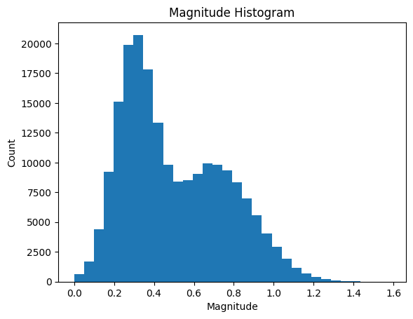
Let’s generate the magnitude histogram using count data.

my_marginal_magnitude_histogram = my_sphere.construct_marginal_magnitude_histogram(
    labelled_vectors, return_fraction=False
)

my_marginal_magnitude_histogram.to_frame()

	0
shell
0	645
1	1693
2	4401
3	9222
4	15096
...	...
27	41
28	20
29	9
30	1
31	3

32 rows × 1 columns

To plot these data as a histogram, we can call the function produce_1d_scalar_histogram() in the plotting module.

ax = vr.plotting.produce_1d_scalar_histogram(
    my_marginal_magnitude_histogram, magnitude_bins
)
ax.set_title("Magnitude Histogram")
ax.set_xlabel("Magnitude")
ax.set_ylabel("Count")

Text(0, 0.5, 'Count')

Note

As shown in the example above, the plot does not include axis labels or a title. Behind the scenes, we use Matplotlib to produce this plot. Make sure to check our their documentation to customise your plots.

This histogram shows the distribution of magnitude values in the data without considering the orientation.

Marginal Direction and Orientation Histograms

In our example in the previous section, we generated direction histograms using a SphereBase with only a single shell. But what if we don’t want to perform the bin assignment again? We can construct the marginal direction or orientation plot using the method SphereBase.construct_marginal_orientation_histogram().

my_marginal_direction_histogram = my_sphere.construct_marginal_orientation_histogram(
    labelled_vectors, return_fraction=False
)

my_marginal_direction_histogram.to_frame()

		0
ring	bin
0	0	7
1	0	14
	1	9
	2	10
	3	7
...	...	...
52	2	7
	3	5
	4	4
	5	3
53	0	8

5806 rows × 1 columns

Similar to the bivariate histogram, we need to get a sphere mesh. To get a single sphere with the faces coloured according to our new histogram, we can use the SphereBase.create_shell_mesh() method.

my_marginal_direction_mesh = my_sphere.create_shell_mesh(
    my_marginal_direction_histogram
)

We can now create a SpherePlotter to plot the direction histogram.

my_marginal_direction_sphere_plotter = vr.plotting.SpherePlotter(
    my_marginal_direction_mesh
)
my_marginal_direction_sphere_plotter.produce_plot()
my_marginal_direction_sphere_plotter.show()

Now we can see the directions of all the vectors, regardless of magnitude.

Conditional Histograms

But now, what if we don’t want to disregard the magnitude completely? Well, VectoRose includes functions for constructing conditional histograms. As with the marginal histograms, we can compute conditional histograms of either variable, either studying the orientation for specific magnitude values or studying the magnitudes for specific orientations. In both cases, VectoRose produces histogram counts similar in structure to the bivariate histogram. The key difference is in the normalisation.

For the conditional magnitude histogram, the counts are normalised by orientation bin, so that adding the frequency values in the same bin across different shells yields a probability of 1.

For the conditional orientation histogram, the counts are normalised by shell, so that adding the frequencies within a single shell yields a probability of 1.

Attention

Unlike the marginal and bivariate cases, the conditional histograms do not offer the possibility of examining count values. Obtaining the count values corresponding to each direction bin or magnitude shell can simply be done by indexing the bivariate histogram.

Important

As you’ll see in the discussion below, VectoRose computes all conditional histograms for shells and orientation bins. So, you don’t actually select the desired magnitudes and orientations before calling the relevant SphereBase methods, but rather after. This is not the only way of computing conditional histograms, but we have included this process for convenience.

Conditional Magnitude Histograms

To study the magnitudes in a specific orientation, we can construct conditional magnitude histograms using the SphereBase.construct_conditional_magnitude_histogram() method. Let’s construct the conditional magnitude histogram for our sample dataset.

my_conditional_magnitude_histogram = my_sphere.construct_conditional_magnitude_histogram(
    labelled_vectors
)

my_conditional_magnitude_histogram.to_frame()

			0
shell	ring	bin
0	0	0	0.0
1	0	0	0.0
2	0	0	0.0
3	0	0	0.0
4	0	0	0.0
...	...	...	...
27	53	0	0.0
28	53	0	0.0
29	53	0	0.0
30	53	0	0.0
31	53	0	0.0

185792 rows × 1 columns

Now we can see that we still have values for every shell and every orientation bin, but the values have been normalised. We can use indexing to extract an individual bin.

Tip

Have an angle in mind that looks interesting based on the spherical axes, but don’t know what bin it corresponds to? If you’re using a TregenzaSphere, you can get the ring and the bin for a specific angle using the TregenzaSphere.get_closest_faces() method.

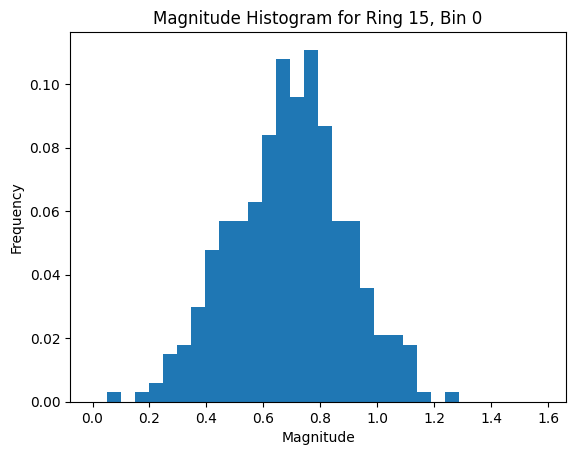
In our case, the bin around \((\phi, \theta) = (50, 0)\) looks interesting. Using TregenzaSphere.get_closest_faces() after some pre-processing, we find that this angle falls in ring 15, bin 0. Let’s extract that bin. Since our histogram has a multi-level index, we need to index by shell, then ring and finally by bin. Since we want all shells, we must included a colon : as the first index.

my_selected_direction_bin = my_conditional_magnitude_histogram[:, 15, 0]

my_selected_direction_bin.to_frame()

	0
shell
0	0.000000
1	0.002994
2	0.000000
3	0.002994
4	0.005988
...	...
27	0.000000
28	0.000000
29	0.000000
30	0.000000
31	0.000000

32 rows × 1 columns

Now, just a sanity check so that you can believe what I said about the normalisation:

my_selected_direction_bin.sum()

np.float64(1.0)

The frequencies do indeed sum up to 1.

Attention

The sum should only ever not equal 1 if there is not a single vector that falls in that orientation, across all shells. In this case, the sum will be equal to 0.

Now, to plot the magnitudes, we can simply call our function produce_1d_scalar_histogram() from plotting, as we did in the marginal case. Remember, we need to pass in the magnitude bins, too!

ax = vr.plotting.produce_1d_scalar_histogram(
    my_selected_direction_bin, magnitude_bins
)
ax.set_title("Magnitude Histogram for Ring 15, Bin 0")
ax.set_xlabel("Magnitude")
ax.set_ylabel("Frequency")

Text(0, 0.5, 'Frequency')

Now, you may be thinking that selecting a single bin is quite narrow. There are a few possible approaches to construct slightly broader conditional histograms. You may select multiple bins, add the frequencies and re-normalise or choose a coarser sphere discretisation. You may also cast a wider net and pre-select vectors within a certain distance of a direction of interest. We will cover these approaches in other examples.

Conditional Direction Histograms

Now, let’s approach the opposite question. Let’s say we are interested in a particular magnitude level and we want to study the orientations of vectors within that magnitude range. We can do this using the method SphereBase.construct_conditional_orientation_histogram(). As we did before, let’s apply this method to our sample data.

my_conditional_orientation_histogram = my_sphere.construct_conditional_orientation_histogram(
    labelled_vectors
)

my_conditional_orientation_histogram.to_frame()

			0
shell	ring	bin
0	0	0	0.0
	1	0	0.0
		1	0.0
		2	0.0
		3	0.0
...	...	...	...
31	52	2	0.0
		3	0.0
		4	0.0
		5	0.0
	53	0	0.0

185792 rows × 1 columns

Let’s say we only want to look at vectors with a magnitude in the bin just below 0.8. First, we need to find what shell that corresponds to. We can do that using a simple search using NumPy’s numpy.searchsorted() function. We exclude the first bin for technical reasons.

desired_shell_index = np.searchsorted(magnitude_bins[1:], 0.8, side="right")

print(f"The desired shell is shell {desired_shell_index}.")

The desired shell is shell 16.

Now that we have the index, we can select the shell.

my_selected_shell_histogram = my_conditional_orientation_histogram[desired_shell_index]

my_selected_shell_histogram.to_frame()

		0
ring	bin
0	0	0.00000
1	0	0.00012
	1	0.00000
	2	0.00012
	3	0.00000
...	...	...
52	2	0.00000
	3	0.00000
	4	0.00000
	5	0.00000
53	0	0.00000

5806 rows × 1 columns

As we did in the magnitude case, let’s run a sanity check to make sure our frequencies add up properly.

my_selected_shell_histogram.sum()

np.float64(1.0)

The selected shell is indeed a true histogram using frequency values.

We now plot it similar to how we plotted the marginal orientation histogram by constructing a mesh and then using a SpherePlotter.

my_conditional_shell_mesh = my_sphere.create_shell_mesh(
    my_selected_shell_histogram
)

my_conditional_sphere_plotter = vr.plotting.SpherePlotter(
    my_conditional_shell_mesh
)
my_conditional_sphere_plotter.produce_plot()
my_conditional_sphere_plotter.show()

This plot shows the distribution of orientations only for the selected vectors. All vectors with a magnitude outside the selected bin are ignored. It is as if we are only looking at one shell of the bivariate histogram and we have normalised the values based on that shell.

Tip

This approach works very well for a single shell. We have provided an additional option to perform a similar normalisation on all shells in the bivariate histogram. When constructing the histogram meshes using the method SphereBase.create_histogram_meshes(), the argument normalise_by_shell can be set to True. In this case, all the values are rescaled relative to the shell maximum. The produced shells all resemble their respective conditional shells, while the face values, all ranging between 0 and 1, can be interpreted as the fraction of the respective shell maximum value achieved.

Summary

At this point, we’ve now seen how to generate many different types of plots using VectoRose.

• The bivariate histogram shows how the magnitude and direction change together using nested spheres.

• The marginal histograms show how one of magnitude or direction change without any regard to the other variable.

• The conditional histograms reveal insight about one of the variables, while the value of the other has been pre-determined.

We have presented the major steps of a simple workflow for constructing the various plots.

Important

While we have presented one simple workflow, this page is by no means exhaustive. There are many different approaches that can be used to select subsets of the vectors for analysis. But, in any case, you will need to use some subclass of SphereBase, so knowing its methods is critical.

At this point, we have covered the basics of visual analysis of non-unit axial and vectorial data. Now, let’s move into the world of statistical analysis. In the next section, we’ll see some statistics that we can compute on our vectorial data. In this next section, the ideas of joint, marginal and conditional histograms and distributions will be important. Make sure that you are comfortable with these concepts before proceeding.