Rotated Layers Example

In all our examples until now, we’ve been considering randomly-generated vectors drawn from probability distributions. Now, let’s consider vectors that have a bit of spatial meaning.

In the study of bone, anisotropy refers to the co-alignment of nearby structures. In this example, we’ll consider the anisotropy of a more idealised assembly: a collection of parallel cylinders arranged in offset layers.

We’ve constructed this assembly using Blender and we’ve computed the anisotropy using the the method introduced by Reznikov et al. [2022], implemented in the Dragonfly 3D World image analysis software.

Before beginning the analysis, let’s look at the data. Here is a rendering of the mesh, as well as the visualisation of the vector field coloured by degree of anisotropy (magnitude) and orientation.

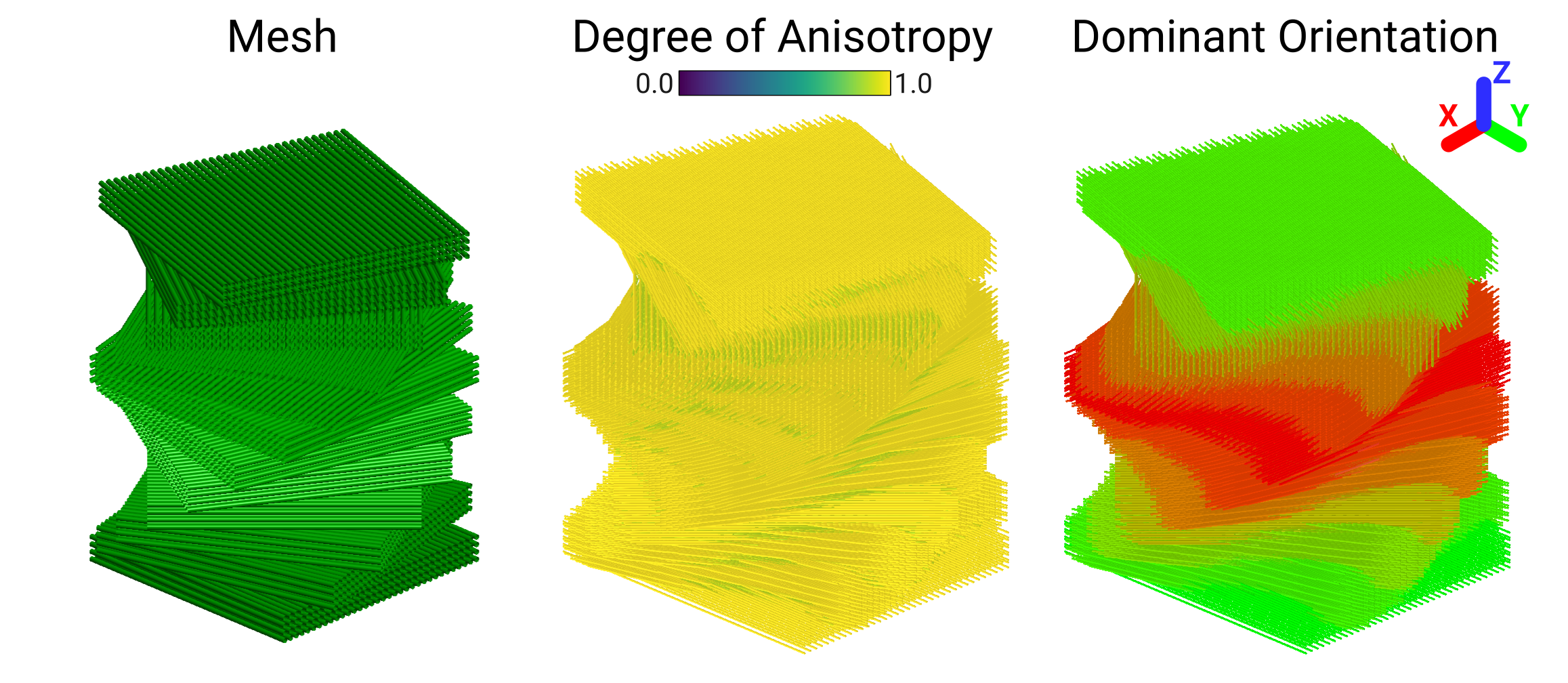
This simulated structure consists of layers of cylinders. Each block of four layers is rotated by 15° relative to the previous one.

Unlike in previous examples, we now have spatial information! The vectors have locations in space, as well as the three components.

Now, we’ll go over how to load the anisotropy data, construct the magnitude, orientation and nested sphere histograms, and compute some statistics using the various tools in VectoRose.

Important

As always, don’t forget to import the vectorose package.

import matplotlib.pyplot as plt
import vectorose as vr

Data Import

Let’s start by importing and preprocessing the vectors. These vectors are found in the file twisted_blocks.npy. These vectors are also bundled in the data module, as SampleData.TWISTED_BLOCKS and so we can access them without downloading any extra files.

For pre-processing, we will remove zero-vectors, convert all the vectors to axes (as anisotropy is an axial quantity) and create symmetric vectors to improve the visualisation.

import vectorose.data

# Load and preprocess the vectors
vectors = vr.data.SampleData.TWISTED_BLOCKS.load()

vectors = vr.util.remove_zero_vectors(vectors)
vectors = vr.util.convert_vectors_to_axes(vectors)

symmetric_vectors = vr.util.create_symmetric_vectors_from_axes(vectors)

Vector Bin Assignment

Before we can construct any histograms, we need to create a sphere representation. In this case, we will use the Fine Tregenza Sphere, represented by FineTregenzaSphere. To ensure that we can perform fine-grain analysis of the degree of anisotropy in our data set, we’ll set the number of magnitude bins to 32. All anisotropy values are between 0 and 1, so we will set our magnitude_range to these values to ensure that the lowest bin has a lower bound of 0 and the highest bin has an upper bound of 1.

sphere = vr.tregenza_sphere.FineTregenzaSphere(
    number_of_shells=32, magnitude_range=(0, 1)
)

labelled_vectors, magnitude_bin_edges = sphere.assign_histogram_bins(symmetric_vectors)

labelled_vectors

	x	y	z	phi	theta	magnitude	shell	ring	bin
0	-52.31424	-53.814232	-0.250002	89.999997	360.000000	1.0	31	26	172
1	-50.81424	-53.814232	-0.250002	89.999997	360.000000	1.0	31	26	172
2	-49.31424	-53.814232	-0.250002	89.999997	360.000000	1.0	31	26	172
3	-47.81424	-53.814232	-0.250002	89.999997	360.000000	1.0	31	26	172
4	-46.31424	-53.814232	-0.250002	89.999997	360.000000	1.0	31	26	172
...	...	...	...	...	...	...	...	...	...
1093345	-28.31424	66.185768	140.750000	90.000000	17.999978	1.0	31	27	8
1093346	-26.81424	66.185768	140.750000	90.000001	17.999955	1.0	31	27	8
1093347	-34.31424	67.685768	140.750000	90.000013	197.999964	1.0	31	27	95
1093348	-32.81424	67.685768	140.750000	90.000008	197.999967	1.0	31	27	95
1093349	-31.31424	67.685768	140.750000	90.000013	197.999967	1.0	31	27	95

1093350 rows × 9 columns

As we can see here, the labelled vectors preserve their spatial coordinates. Thanks to this feature, we could easily extract all vectors with a specific direction.

Magnitude Histogram

Now, let’s begin constructing the histograms. We’ll start with the magnitude histogram, showing the degree of anisotropy.

magnitude_histogram = sphere.construct_marginal_magnitude_histogram(
    labelled_vectors, return_fraction=True
)

ax = plt.axes()
ax = vr.plotting.produce_1d_scalar_histogram(
    magnitude_histogram, magnitude_bin_edges, ax=ax
)
ax.set_title("Offset Sheets - Degree of Anisotropy")
ax.set_xlabel("Degree of Anisotropy")
ax.set_ylabel("Frequency")
plt.show()

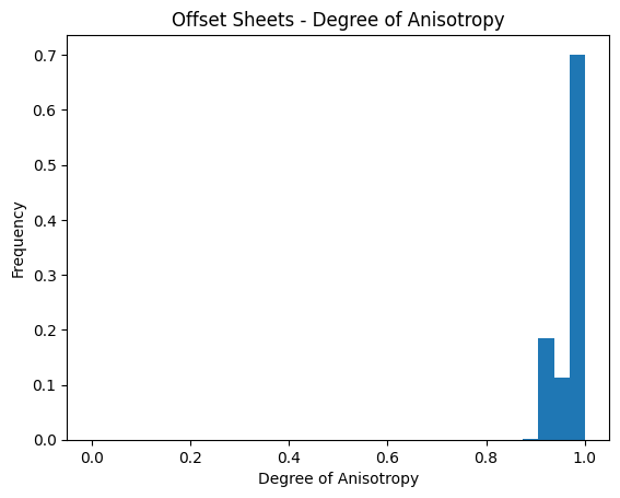
This histogram shows that the degree of anisotropy is very high for most of the vectors. This histogram gives us a global picture of the degree of anisotropy, it does not give us any insight into the anisotropy orientations. To understand these orientations, we can compute a different type of histogram.

Orientation Histogram

Now, let’s construct the orientation histogram and visualise it in 3D. Remember that to visualise orientation plots in 3D, we need to create a SpherePlotter object and provide it histogram meshes.

orientation_histogram = sphere.construct_marginal_orientation_histogram(
    labelled_vectors, return_fraction=True
)

orientation_mesh = sphere.create_shell_mesh(orientation_histogram)

orientation_sphere_plotter = vr.plotting.SpherePlotter(orientation_mesh)
orientation_sphere_plotter.produce_plot()
orientation_sphere_plotter.show()

2026-05-21 05:25:53.294 (   2.274s) [    76B56454AB80]vtkXOpenGLRenderWindow.:1458  WARN| bad X server connection. DISPLAY=

This spherical histogram shows where there anisotropy axes are pointing. Most of them appear to be very close to the equator. This makes sense considering the layout of the cylinders above. The gaps along the equator correspond to angles not present due to the 15° angular increments. While this histogram provides insight into the orientations, we lose all information about the magnitude.

Now, for one last thing. Now that we’re done with our 3D plot, we should close the plotter to free up computational resources.

orientation_sphere_plotter.close()

Nested Spherical Histogram

What if we want to study both the magnitudes and orientations together? To do this, we can construct nested spherical histograms.

Warning

Unfortunately, this plot won’t work very well in the browser-rendered version of this example. Make sure to run this example in a Jupyter notebook to see the results.

bivariate_histogram = sphere.construct_histogram(labelled_vectors, return_fraction=True)
bivariate_histogram_meshes = sphere.create_histogram_meshes(
    bivariate_histogram, magnitude_bin_edges, normalise_by_shell=False
)

bivariate_sphere_plotter = vr.plotting.SpherePlotter(bivariate_histogram_meshes)
bivariate_sphere_plotter.produce_plot()
bivariate_sphere_plotter.show()

This histogram provides a combination of magnitude and orientation. By adjusting the sliders, we can see how the orientations change for different magnitude levels. In this example, there will be little change. In other examples, such as the one shown in the Quick Start, the appearance can change quite a bit from shell to shell.

As before, let’s close the plotter to free up resources.

bivariate_sphere_plotter.close()

Statistics

We can also compute statistics using the vectors. Note that to compute statistics, we should use the axes stored in the vectors variable and not the duplicated vectors stored in symmetric_vectors.

labelled_vectors, magnitude_bin_edges = sphere.assign_histogram_bins(vectors)

labelled_vectors

	x	y	z	phi	theta	magnitude	shell	ring	bin
0	-52.31424	-53.814232	-0.250002	89.999997	360.000000	1.0	31	26	172
1	-50.81424	-53.814232	-0.250002	89.999997	360.000000	1.0	31	26	172
2	-49.31424	-53.814232	-0.250002	89.999997	360.000000	1.0	31	26	172
3	-47.81424	-53.814232	-0.250002	89.999997	360.000000	1.0	31	26	172
4	-46.31424	-53.814232	-0.250002	89.999997	360.000000	1.0	31	26	172
...	...	...	...	...	...	...	...	...	...
546670	-28.31424	66.185768	140.750000	90.000000	197.999978	1.0	31	26	95
546671	-26.81424	66.185768	140.750000	89.999999	197.999955	1.0	31	26	95
546672	-34.31424	67.685768	140.750000	89.999987	17.999964	1.0	31	26	8
546673	-32.81424	67.685768	140.750000	89.999992	17.999967	1.0	31	26	8
546674	-31.31424	67.685768	140.750000	89.999987	17.999967	1.0	31	26	8

546675 rows × 9 columns

Now, we can compute a number of statistical results for all vectors or a subset of them.

Mean Resultant Vector

The mean resultant vector provides an indication of a dominant orientation (if one is present) and a rough idea of whether the vectors are co-aligned.

unit_vectors = sphere.convert_vectors_to_cartesian_array(
    labelled_vectors, create_unit_vectors=True
)

mean_resultant_vector = vr.stats.compute_resultant_vector(
    unit_vectors, compute_mean_resultant=True
)

mean_resultant_spherical_coordinates = vr.util.compute_spherical_coordinates(
    mean_resultant_vector, use_degrees=True
)

mean_phi = mean_resultant_spherical_coordinates[0]
mean_theta = mean_resultant_spherical_coordinates[1]
mean_resultant_length = mean_resultant_spherical_coordinates[-1]

print(f"Mean resultant length: {mean_resultant_length}")
print(f"Mean resultant orientation: ({mean_phi}\u00b0, {mean_theta}\u00b0).")

Mean resultant length: 0.11191115158735532
Mean resultant orientation: (89.866605957703°, 298.64377408932523°).

The low value of the mean resultant length suggests that there is not a single dominant orientation. Unfortunately, this value doesn’t tell us much else about the shape of the distribution. Thankfully, there are other metrics that are more helpful…

Woodcock’s Parameters

Looking at the images of the anisotropy field and the spherical histograms, it seems that we have a girdle distribution. To verify this numerically, we can compute Woodcock’s shape and strength parameters.

orientation_matrix_eig_result = vr.stats.compute_orientation_matrix_eigs(unit_vectors)

woodcock_parameters = vr.stats.compute_orientation_matrix_parameters(
    orientation_matrix_eig_result.eigenvalues
)

print(f"Shape parameter: {woodcock_parameters.shape_parameter}.")
print(f"Strength parameter: {woodcock_parameters.strength_parameter}.")

Shape parameter: 0.004949952388512854.
Strength parameter: 11.324244405217284.

The very low shape parameter supports the claim that the data follow a girdle distribution. The very high strength parameter suggests that the data are very compact with little noise.

Summmary

In this section, we’ve seen a walk-through of a sample analysis pipeline for structural anisotropy vectors. We preprocessed the vectors, assigned them to bins, and constructed a variety of histograms.