Loading Vectors into VectoRose#
The previous section introduced axial and vectorial data. VectoRose is a Python package that can be used to visualise and analyse these data. But, before the data can be examined, the vectors must be loaded into VectoRose.
This page describes how vectors must be formatted and how to import them into VectoRose. Unlike images, which have very well-defined standards, vectorial data have yet to be widely standardised. We have tried to define simple, intuitive formats for representing vectorial data.
Data Formats and Layout#
VectoRose accepts axial and vectorial data in three formats:
Binary NumPy files (
*.npy)Comma-separated value files (
*.csvor*.txt)Excel spreadsheets (
*.xlsx)
The data must be arranged so that each row represents a single vector, and the columns represent the vector components. This diagram illustrates how the file should be organised:
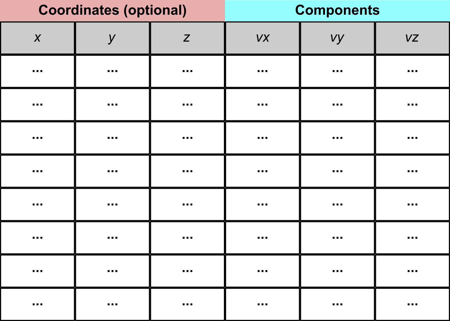
If the provided vectors contain spatial information, the first three columns are assumed to represent the vector positions in space, while the last three columns are assumed to represent the vector components. While these settings are the default, they can be easily customised to accommodate files produced by other software tools.
Attention
While it is possible to configure these options when loading a file, once a collection of vectors is open in VectoRose, these are the conventions that are followed.
NumPy Arrays#
NumPy binary array files (see here for more detail) are a flexible, efficient way of storing multidimensional arrays. The important trade-off is that the file format is binary, and so you can’t open these files in a text editor.
Higher-dimensional Arrays#
Unlike spreadsheets and text-based files, the information stored in NumPy arrays are not restricted to two dimensions. NumPy files can easily store arrays of any dimension. An example of a higher dimensional array is a vector field. Since a vector is defined at each position in 3D space, it may be more intuitive to store these data in a 4D array, where three of the dimensions represent the spatial location and the fourth is used to distinguish the vector components.
Warning
Currently, only *.npy files can be imported. To import an array stored in
a compressed *.npz file, extract the constituent arrays and load the
specific *.npy file extracted.
CSV Files#
CSV files are a plain-text format which represent data as a 2D table.
Each line in the file represents a table row. Within a row, columns are
separated by a specific character, such as a comma (,), a tab (\t), a
space ( ) or a semicolon (;). As these files are text-based, they are
relatively lightweight and can easily be opened with a wide variety of
editing software[1].
Excel Spreadsheets#
Excel spreadsheets are a more sophisticated XML-based format for storing multiple 2D tables as sheets containing rows and columns. Similar to the other formats described, rows represent different vectors and columns represent different vector components.
Warning
VectoRose can only open the newer *.xlsx files. The older *.xls
spreadsheets may not be supported.
Importing Vectors into VectoRose#
Once we have vectors in one of the file formats described above, we can load these vectors into Python using VectoRose.
Before trying to load your vectors, you must import the vectorose
package into the Python interpreter:
import vectorose as vr
Tip
To save some time writing code, we recommend using vr as a shorthand for
vectorose.
Vectors are imported using the function
vectorose.io.import_vector_field(). For example, if your vectors are
in a NumPy array file called two_clusters.npy, we can load the vectors
by writing:
import vectorose as vr

vectors = vr.io.import_vector_field("two_clusters.npy")

vectors
array([[ 0.01330902,  0.06486094, -0.08154041],
       [ 0.19911095,  0.06809676, -0.02230348],
       [ 0.14568445,  0.08995054,  0.06688315],
       ...,
       [-0.0377645 ,  0.35891606,  0.6731566 ],
       [-0.13033349,  0.56234415,  0.27104764],
       [-0.03287074,  0.60723468,  0.63249369]], shape=(200000, 3))
We can now see that we have an array of vectors available to process and analyse.
There are a number of parameters that can control how the vectors are loaded. The most important parameters are:
component_columnsIndicate the columns containing the
x,y,zvector components. By default, the last three columns are considered.location_columnsIndicate the columns containing the
x,y,zpositions of the vectors in space, in the case of a vector field. If this is set toNone, then the location coordinates are ignored. By default, the first three columns are considered.separatorWhen reading vectors from a CSV file, indicate what character is used to separate the columns.
contains_headersIndicate whether the first row of the file contains column headers, which will be discarded.
sheetWhen reading vectors from an Excel file, indicate the name or position of the sheet to read.
Regardless of the file type, this function creates a 2D NumPy array with
n rows, corresponding to the number of vectors, and either 3 or 6
columns, depending on whether the location coordinates are read.
Pre-processing Vectors#
Once the vectors are read, there are a number of important pre-processing steps that can be performed:
vectorose.util.remove_zero_vectors()Remove all vectors with a magnitude of zero from the list.
vectorose.util.convert_vectors_to_axes()Flip all vectors having a negative
z-component to ensure that all orientations are contained within the upper unit hemisphere.vectorose.util.create_symmetric_vectors_from_axes()When analysing axial data, generate a pair of antiparallel vectors for each vector in the list.
vectorose.util.normalise_vectors()Return a set of unit vectors having the same orientations/directions as the loaded data.
Example#
We have a collection of vectors in two_clusters.csv.
Take a look at this file… the columns are separated by commas and the
first row is a header, and there are no spatial
coordinates present.
Let’s load these vectors, remove any zero-vectors and convert these vectors into an axial representation. Here’s how we can perform this task:
import vectorose as vr

# Load the vectors from the CSV file
vectors = vr.io.import_vector_field(
    "two_clusters.csv", contains_headers=True, location_columns=None, separator=","
)

print(f"We have loaded {vectors.shape[0]} vectors from the file.")

# Remove zero-magnitude vectors
vectors = vr.util.remove_zero_vectors(vectors)
print(f"We have {vectors.shape[0]} non-zero vectors.")

# Convert to axial data
vectors = vr.util.convert_vectors_to_axes(vectors)

vectors
We have loaded 300000 vectors from the file.
We have 200000 non-zero vectors.
array([[-0.1994052 ,  0.30333967,  0.5381077 ],
       [-0.21734826, -0.24813696,  0.21420199],
       [-0.01614593, -0.18969616,  0.06309708],
       ...,
       [-0.31431377, -0.12350598,  0.223283  ],
       [ 0.00408248, -0.11394966,  0.26480249],
       [ 0.26338823,  0.26370685,  0.37286224]], shape=(200000, 3))
We can now see that we’ve loaded the vectors, and we’ve managed to prune quite a few zero-vectors that we had in our dataset.
See also
For more details about importing vector fields, check out the
documentation on vectorose.io and for more on pre-processing,
consult the page on vectorose.util.
Bundled Examples#
To make the process of loading sample data easier when following along with
the documentation, we have bundled three sample datasets that can be loaded
directly in VectoRose without needing to download any additional files.
These datasets can be accessed via the class data.SampleData.
Attention
The sample data are found in the vectorose.data module, which is not
automatically imported. You must explicitly import the data
submodule using:
import vectorose.data
Even if the vr alias is used for vectorose, the full package name
should still be used for this import.
In the case of the two_clusters dataset, we can open the vectors easily
using the SampleData.load() method of the object
SampleData.TWO_CLUSTERS:
import vectorose.data

vectors = vr.data.SampleData.TWO_CLUSTERS.load()

print(f"We have loaded {vectors.shape[0]} vectors from the file.")

# Remove zero-magnitude vectors
vectors = vr.util.remove_zero_vectors(vectors)
print(f"We have {vectors.shape[0]} non-zero vectors.")

# Convert to axial data
vectors = vr.util.convert_vectors_to_axes(vectors)

vectors
We have loaded 200000 vectors from the file.
We have 200000 non-zero vectors.
array([[-0.01330902, -0.06486094,  0.08154041],
       [-0.19911095, -0.06809676,  0.02230348],
       [ 0.14568445,  0.08995054,  0.06688315],
       ...,
       [-0.0377645 ,  0.35891606,  0.6731566 ],
       [-0.13033349,  0.56234415,  0.27104764],
       [-0.03287074,  0.60723468,  0.63249369]], shape=(200000, 3))
But, loading vectors is just the beginning! Now that we know how to load and pre-process vectors, we can begin with data visualisation.