Quick Start#
Welcome to VectoRose! This document is intended to help you get up and running quickly with our package. If you want a more thorough introduction, make sure to keep reading the next pages of this manual. This page is meant to provide an overview of the features present in VectoRose, as well as a quick example pipeline, without diving so deeply into the theory behind everything.
In this page, we’ll be using a sample dataset of simulated vectors. These
vectors, stored in cluster_girdle.npy, are from a simulated dataset. These vectors are also
bundled with VectoRose as an example, and don’t need to be downloaded
separately. We’ll analyse these vectors quite closely during this example.
What is VectoRose?#
VectoRose is a Python package for analysing vectorial and axial data. Unlike existing tools, these vectors are not required to have unit length. VectoRose contains tools for two main purposes: plotting and statistical analysis. We’ll scratch the surface of both of these in this guide.
Three different types of histograms can be constructed using VectoRose:
1D scalar histograms to visualise vector magnitudes
Spherical histograms to visualise vector directions
Nested spherical histograms to visualise all combinations of magnitude and orientation.
In this example, we’ll see how to generate and plot each of these.
Can I use VectoRose in my research?#
Yes! VectoRose is open-source and licensed under the MIT License. Anyone can use VectoRose for any purpose and even modify and further develop it. The only requirement is that you attribute us as the original authors. We also request that you cite [Rudski et al., 2025] if you publish any articles that use our tool.
Note
Interested in modifying and extending VectoRose? Check out our Contributing guide to get started.
Installing VectoRose#
Installing VectoRose is very straightforward. The only requirement is that you have Python installed. At the command line, type the following to install VectoRose:
pip install vectorose
There are more advanced installation options available, of course. Make sure to check out our installation page for more details.
Importing VectoRose#
Now, let’s get to the actual code! Make sure you have Python open. To
start, let’s import the vectorose package. To make things easier, we use
the alias vr when we import.
import vectorose as vr
We can now use all the VectoRose functionality.
Extra Configuration#
To improve how this example appears in our rendered HTML web page, we can configure a couple of extra options.
First, to ensure that our interactive 3D plots appear, we need to call
pyvista.set_jupyter_backend() to change the PyVista rendering backend
to "html".
import pyvista as pv
import platform
pv.set_jupyter_backend("html")
We can also change how our data tables produced using Pandas appear using
pandas.options.
We’ll just control the number of rows that appear, but there are many other
options that can be changed.
import pandas as pd
pd.options.display.max_rows = 20
We’re now ready to dive into our example.
Loading and Preprocessing the Vectors#
Let’s begin by loading our vectors into Python. To do this, we can use the
function vectorose.io.import_vector_field().
vectors = vr.io.import_vector_field("cluster_girdle.npy", location_columns=None)
vectors
array([[-0.01315509, 0.04643773, 0.09329196],
[ 0.04506704, 0.14403199, 0.14833588],
[ 0.04875124, 0.15409187, 0.08756384],
...,
[ 0.061444 , -0.48235211, -0.40355562],
[-0.13128825, 0.38257552, 0.40000009],
[-0.31063193, -0.50151858, -0.35539716]], shape=(150000, 3))
Tip
As was mentioned above, you don’t need to download the vector to be able to
analyse them in this example. We have included a few sample datasets with
VectoRose, including the cluster_girdle vectors, in the
:class:.data.SampleData class. To load the cluster girdle dataset,
simply run the following code:
import vectorose.data
vectors = vr.data.SampleData.CLUSTER_GIRDLE.load()
We show both methods to illustrate how to load your own data into VectoRose.
Before doing any of our analysis, we must remove the zero-magnitude vectors
using util.remove_zero_vectors().
vectors = vr.util.remove_zero_vectors(vectors)
# Now, let's look at the vectors
vectors
array([[-0.01315509, 0.04643773, 0.09329196],
[ 0.04506704, 0.14403199, 0.14833588],
[ 0.04875124, 0.15409187, 0.08756384],
...,
[ 0.061444 , -0.48235211, -0.40355562],
[-0.13128825, 0.38257552, 0.40000009],
[-0.31063193, -0.50151858, -0.35539716]], shape=(150000, 3))
Tip
There are additional pre-processing steps available. Make sure to check out
the functions in vectorose.util to see other options. The loading
process is covered in more detail in Loading Vectors into VectoRose.
Constructing and Visualising Histograms#
In this section, we’ll give an overview on constructing histograms using VectoRose. For more in-depth discussion, see the pages on Histogram Plotting and Advanced Histogram Plotting. There are three major types of histograms that can be constructed using VectoRose:
Nested spherical histograms - provide insight into magnitude and direction together.
Magnitude histograms - provide insight into magnitude alone.
Direction histograms - provide insight into direction alone.
We’ll see how to construct each of these histograms for our sample data.
Data Binning#
The first step to construct a histogram is to bin the data. To do this, we
need a representation of a sphere. In VectoRose, this can be obtained using
a TriangleSphere or one of our TregenzaSphere
subclasses. In our example, we’ll use a FineTregenzaSphere. This
discretised sphere contains 5806 patches in 54 rings. To study the
magnitude, we’ll construct 32 bins, which will be represented as the nested
spherical shells.
We’ll then assign the bins using SphereBase.assign_histogram_bins().
sphere = vr.tregenza_sphere.FineTregenzaSphere(number_of_shells=32)
labelled_vectors, magnitude_bins = sphere.assign_histogram_bins(
vectors
)
# Let's look at the labelled vectors
labelled_vectors
| phi | theta | magnitude | shell | ring | bin | |
|---|---|---|---|---|---|---|
| 0 | 27.355028 | 344.183391 | 0.105038 | 3 | 8 | 73 |
| 1 | 45.494371 | 17.374695 | 0.211612 | 6 | 14 | 6 |
| 2 | 61.551662 | 17.556214 | 0.183816 | 5 | 18 | 7 |
| 3 | 41.075034 | 29.278268 | 0.283404 | 8 | 12 | 9 |
| 4 | 40.949336 | 49.701711 | 0.301634 | 9 | 12 | 15 |
| ... | ... | ... | ... | ... | ... | ... |
| 149995 | 60.578409 | 116.382555 | 0.711134 | 21 | 18 | 49 |
| 149996 | 54.439695 | 316.886418 | 0.700464 | 21 | 16 | 124 |
| 149997 | 129.690457 | 172.740525 | 0.631899 | 19 | 38 | 64 |
| 149998 | 45.318759 | 341.059343 | 0.568859 | 17 | 14 | 121 |
| 149999 | 121.066580 | 211.773357 | 0.688709 | 21 | 36 | 86 |
150000 rows × 6 columns
Nested Spherical Histograms#
To construct the nested spherical histogram, we can use the method
SphereBase.construct_histogram() for our sphere representation.
histogram = sphere.construct_histogram(labelled_vectors)
histogram.to_frame()
| frequency | |||
|---|---|---|---|
| shell | ring | bin | |
| 0 | 0 | 0 | 0.0 |
| 1 | 0 | 0.0 | |
| 1 | 0.0 | ||
| 2 | 0.0 | ||
| 3 | 0.0 | ||
| ... | ... | ... | ... |
| 31 | 52 | 2 | 0.0 |
| 3 | 0.0 | ||
| 4 | 0.0 | ||
| 5 | 0.0 | ||
| 53 | 0 | 0.0 |
185792 rows × 1 columns
We can then visualise the histogram by constructing the shell meshes using
SphereBase.create_histogram_meshes() and the show them in 3D using
SpherePlotter from the plotting module.
sphere_meshes = sphere.create_histogram_meshes(histogram, magnitude_bins)
sphere_plotter = vr.plotting.SpherePlotter(sphere_meshes)
sphere_plotter.produce_plot()
sphere_plotter.show()
2026-03-18 00:44:23.092 ( 3.897s) [ 7C8B90F85B80]vtkXOpenGLRenderWindow.:1458 WARN| bad X server connection. DISPLAY=
Danger
Remember to call the SpherePlotter.produce_plot() method to add the
spheres to the plot before showing it.
Now we can see the constructed meshes, and we also have some sliders that let us change which shell is visible. This may not appear in the static HTML version of the documentation, so we’re exporting and embedding a video and a screenshot here showing the different shells.
# Make sure our output path exists
import os
output_path = "./assets/quickstart/"
if not os.path.exists(output_path):
os.mkdir(output_path)
sphere_plotter.export_screenshot(
os.path.join(output_path, "nested_spheres.png"),
transparent_background=False,
)
sphere_plotter.produce_shells_video(
os.path.join(output_path, "nested_spheres.mp4"),
quality=5,
fps=4,
boomerang=True,
add_shell_text=True
)
See also
For more information on exporting images and videos from plots, check out
the following SpherePlotter methods.
SpherePlotter.export_screenshot()Export raster screenshots of the 3D plot.
SpherePlotter.export_graphic()Export vector screenshots of the 3D plot (raster image + text).
SpherePlotter.produce_shells_video()Export video going through the nested shells of a histogram plot.
SpherePlotter.produce_rotating_video()Export video of the spherical histogram rotating.
Looking at our series of nested spheres, we see that there are two major patterns in the data. At the higher magnitude levels, represented by the outer shells, we have a ring of vectors, known as a girdle. At the lower magnitude levels, we have a single bright spot of vectors, known as a cluster. These patterns are special, and quite common in directional statistics [see Fisher et al., 1993, Mardia and Jupp, 2000, for more information].
Magnitude Histograms#
To construct the magnitude histogram with 32 bins, we can use the same
sphere representation. We first get the histogram bin counts using the
SphereBase.construct_marginal_magnitude_histogram() method.
magnitude_histogram = sphere.construct_marginal_magnitude_histogram(
labelled_vectors
)
magnitude_histogram.to_frame()
| 0 | |
|---|---|
| shell | |
| 0 | 0.001147 |
| 1 | 0.002040 |
| 2 | 0.003853 |
| 3 | 0.007633 |
| 4 | 0.013447 |
| ... | ... |
| 27 | 0.001193 |
| 28 | 0.000407 |
| 29 | 0.000140 |
| 30 | 0.000033 |
| 31 | 0.000020 |
32 rows × 1 columns
To visualise the histogram, we can use the function
produce_1d_scalar_histogram() in the plotting module. To
customise the plot, we can use all the usual tricks from matplotlib.
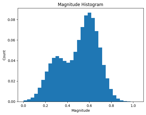
ax = vr.plotting.produce_1d_scalar_histogram(magnitude_histogram, magnitude_bins)
ax.set_title("Magnitude Histogram")
ax.set_xlabel("Magnitude")
ax.set_ylabel("Count")
Text(0, 0.5, 'Count')
Attention
Don’t forget to pass the magnitude bin edges to the function
produce_1d_scalar_histogram()!
Based on this plot, we have a bimodal distribution of magnitudes. Each mode corresponds to one of the two features (girdle and cluster) we described earlier.
Direction Histograms#
To construct the direction histogram, we can call the method
SphereBase.construct_marginal_orientation_histogram() on our sphere
representation.
orientation_histogram = sphere.construct_marginal_orientation_histogram(
labelled_vectors
)
orientation_histogram.to_frame()
| 0 | ||
|---|---|---|
| ring | bin | |
| 0 | 0 | 0.000060 |
| 1 | 0 | 0.000093 |
| 1 | 0.000087 | |
| 2 | 0.000040 | |
| 3 | 0.000013 | |
| ... | ... | ... |
| 52 | 2 | 0.000000 |
| 3 | 0.000000 | |
| 4 | 0.000000 | |
| 5 | 0.000000 | |
| 53 | 0 | 0.000000 |
5806 rows × 1 columns
To visualise the histogram, we can use an approach similar to the nested
spheres approach. The key difference is that we construct a single mesh
using the SphereBase.create_shell_mesh() method. We can then
visualise this mesh using a SpherePlotter like above. We’ve also
added spherical axes using SpherePlotter.add_spherical_axes() to
show the \(\phi\) and \(\theta\) axes in 3D.
orientation_mesh = sphere.create_shell_mesh(orientation_histogram)
sphere_plotter = vr.plotting.SpherePlotter(orientation_mesh)
sphere_plotter.produce_plot()
sphere_plotter.add_spherical_axes()
sphere_plotter.show()
To share these results, we can export a video of the spherical histogram
rotating about its axis using
SpherePlotter.produce_rotating_video(). We can also export a single
still frame using SpherePlotter.export_screenshot(), as before.
sphere_plotter.export_screenshot(
"./assets/quickstart/orientation_histogram.png",
transparent_background=False,
)
sphere_plotter.produce_rotating_video(
"./assets/quickstart/orientation_histogram.mp4",
quality=5,
fps=12,
number_of_frames=36,
hide_sliders=True
)
Using this spherical histogram, we can see that the two patterns, the girdle and the cluster, overlap. However, the nested spherical histograms above illustrate that these are indeed distinct patterns, separated by differences in magnitude.
Tip
Directions and orientations can also be visualised using polar histograms, as described in the page on Histogram Plotting.
Statistics#
In addition to visualising vectorial data, VectoRose also allows computing
directional statistics on the loaded vectors. These statistics are
explained in detail in our Statistics Overview page.
The functions necessary for performing directional statistics are defined
in the module stats.
Directional statistics can be computed on any collection of unit vectors, that is, vectors with a magnitude equal to 1. This set of vectors may be obtained from all vectors, representing the marginal orientation distribution, or from a subset of vectors depending on their magnitude, representing a conditional orientation distribution. We will do both in this example.
We’ve mentioned that our data show two patterns: a girdle in the higher magnitude shells and a cluster in the lower magnitude shells. These two patterns overlap in the marginal orientation histogram.
To quantitatively describe these patterns, we can use Woodcock’s shape and strength parameters [Woodcock, 1977]. These parameters are described in more detail in our Statistics Overview page. The main idea is that we compute two parameters:
Shape parameter: a value between 0 and 1 reflects a girdle, a value greater than 1 represents a cluster and a value equal to 1 represents something in between.
Strength parameter: a large value represents a compact distribution, while a small value represents a diffuse distribution.
These parameters are computed using the eigenvalues of the orientation matrix defined by these vectors (see Statistics Overview).
Since we suspect we have a girdle and a cluster here, let’s compute these
parameters for our distribution. We first need to compute the eigenvalues
of the orientation matrix for our set of vectors using the function
compute_orientation_matrix_eigs() and then we can compute the
shape and strength parameters using the function
compute_orientation_matrix_parameters().
Let’s start with the marginal orientation distribution. This considers all
the vectors. We must convert them first to unit vectors. We can do this
either using util.normalise_vectors() or
SphereBase.convert_vectors_to_cartesian_array(). In this example,
we’ll use the latter.
Warning
If using SphereBase.convert_vectors_to_cartesian_array(), remember
to set create_unit_vectors=True when calling the function.
unit_vectors_all = sphere.convert_vectors_to_cartesian_array(
labelled_vectors, create_unit_vectors=True
)
orientation_matrix_eig_result = vr.stats.compute_orientation_matrix_eigs(
unit_vectors_all
)
eigenvalues = orientation_matrix_eig_result.eigenvalues
woodcock_parameters = vr.stats.compute_orientation_matrix_parameters(
eigenvalues
)
print(f"The marginal distribution has a shape parameter of "
f"{woodcock_parameters.shape_parameter} and a strength parameter of "
f"{woodcock_parameters.strength_parameter}.")
The marginal distribution has a shape parameter of 0.2609003142894843 and a strength parameter of 2.8066647895003305.
We can now do the same for our conditional shells. We can isolate individual shells, or iterate over every shell. Let’s do the same operation for each shell and print out the values on the screen.
We can extract the vectors using our labelled_vectors from before with a
bit of data indexing thanks to Pandas.
number_of_shells = sphere.number_of_shells
for i in range(number_of_shells):
shell_vectors = labelled_vectors[labelled_vectors["shell"] == i]
shell_unit_vectors = sphere.convert_vectors_to_cartesian_array(
shell_vectors, create_unit_vectors=True
)
orientation_matrix_eig_result = vr.stats.compute_orientation_matrix_eigs(
shell_unit_vectors
)
eigenvalues = orientation_matrix_eig_result.eigenvalues
woodcock_parameters = vr.stats.compute_orientation_matrix_parameters(
eigenvalues
)
print(f"Shell {i}: shape parameter {woodcock_parameters.shape_parameter};"
f" strength parameter {woodcock_parameters.strength_parameter}.")
Shell 0: shape parameter 25.12435528074365; strength parameter 2.8393889711984595.
Shell 1: shape parameter 36.472114144210025; strength parameter 2.682660031787996.
Shell 2: shape parameter 29.20064516856242; strength parameter 2.7340549528918223.
Shell 3: shape parameter 38.87213972767684; strength parameter 2.6839707241162234.
Shell 4: shape parameter 47.827877508762626; strength parameter 2.6486200553207344.
Shell 5: shape parameter 90.40650654533775; strength parameter 2.6721699776098764.
Shell 6: shape parameter 85.48549699103968; strength parameter 2.6376216354004134.
Shell 7: shape parameter 57.46206156463621; strength parameter 2.6511187382981283.
Shell 8: shape parameter 28.164852712707187; strength parameter 2.6675378607149853.
Shell 9: shape parameter 12.297961046931214; strength parameter 2.6568265808519347.
Shell 10: shape parameter 4.848370925580512; strength parameter 2.6485200870576184.
Shell 11: shape parameter 1.9930068891977066; strength parameter 2.692893277342888.
Shell 12: shape parameter 0.8289137701070531; strength parameter 2.710457149767289.
Shell 13: shape parameter 0.3583624873269097; strength parameter 2.8289930105980794.
Shell 14: shape parameter 0.14054286922688838; strength parameter 2.8547244415286657.
Shell 15: shape parameter 0.05416879030753901; strength parameter 2.922072797979258.
Shell 16: shape parameter 0.023338819837240506; strength parameter 2.933875900281005.
Shell 17: shape parameter 0.006298357768713872; strength parameter 2.956890987727486.
Shell 18: shape parameter 0.0031870445707900793; strength parameter 2.9629082484862685.
Shell 19: shape parameter 0.006978268802916053; strength parameter 2.9794790897853494.
Shell 20: shape parameter 0.006731869159026684; strength parameter 2.9721240779143883.
Shell 21: shape parameter 0.008161184278272168; strength parameter 2.9711166394101465.
Shell 22: shape parameter 0.010867925079779378; strength parameter 3.0008558412537547.
Shell 23: shape parameter 0.014192859441873429; strength parameter 2.9914162458598472.
Shell 24: shape parameter 0.025202116671733266; strength parameter 3.030529808115784.
Shell 25: shape parameter 0.01269322427259286; strength parameter 2.95714883064019.
Shell 26: shape parameter 0.016460485365784455; strength parameter 2.9696376500659807.
Shell 27: shape parameter 0.040547110174433826; strength parameter 2.905699161920147.
Shell 28: shape parameter 0.11794758498654302; strength parameter 2.8511165457986443.
Shell 29: shape parameter 0.12155176671500664; strength parameter 4.0193467428032.
Shell 30: shape parameter 0.22085222874649002; strength parameter 4.3393343016069235.
Shell 31: shape parameter 0.18984115264444837; strength parameter 4.7591310958611235.
We can see that as we change which window of magnitude is being considered, the shape and strength parameters change. In the lower magnitude shells, we compute very high values for the shape parameter, reflecting the cluster. In the higher magnitude shells, we have very low shape parameter values, reflecting the girdle distribution. In all cases, the strength parameter is quite high, representing a compact distribution.
Tip
Shape and strength parameter are by far not the only values that we can compute to understand the shape and distribution of orientations. Make sure to check out our Statistics Overview for a more thorough description of the analyses that can be performed and the insights that can be obtained from collections of vectors.
Next Steps#
This is the end of our Quick Start guide. This guide is not meant to be a comprehensive overview; it’s just a first look to help you get up and running. If you want to explore VectoRose in more depth, we recommend continuing to read this Users’ Guide.
In addition to our resources, it can also help to familiarise yourself with NumPy and pandas. VectoRose uses these packages extensively and knowing more about them will enable you to do more advanced operations, including:
Exporting and importing histograms from files.
Filtering vectors based on magnitude, orientation and angular distance.
Developing other statistical functionality.
We hope that this first guide has been helpful. If you encounter any difficulties or bugs using VectoRose, make sure to open a GitHub issue at bzrudski/vectorose#issues. Welcome to VectoRose!